Data Warehousing Fundamentals & Kimball Dimensional Modeling
With the rapid rise of modern Lakehouses and cloud-native object storage, it is easy to assume that traditional data warehousing is a relic of the past. But the truth is, while the storage layer has evolved, the logic of how we structure data for human understanding hasn't changed. If you want to build scalable, high-performance analytical systems, mastering Kimball’s dimensional modeling isn't just optional, it is the absolute foundation of data engineering.
This is a lengthy post, hoping to cover all the foundational data warehousing concepts.
Lets start by going over basic term and concepts used in data warehousing.
Basic terms and concepts
OLTP vs OLAP
| Feature | OLTP (Online Transaction Processing) | OLAP (Online Analytical Processing) |
|---|---|---|
| Purpose | Day-to-day operations | Data analysis and decision support |
| Data Model | Highly normalized (3NF) | Dimensional (Star/Snowflake) |
| Operations | Insert, Update, Delete | Select (Read-heavy) |
| Users | Clerks, Cashiers, End-users | Analysts, Executives |
| Data Volume | Small, recent transactions | Historical, large volumes |
| Response Time | Milliseconds | Seconds to minutes |
| Examples | Banking, eCommerce apps | BI tools, dashboards |
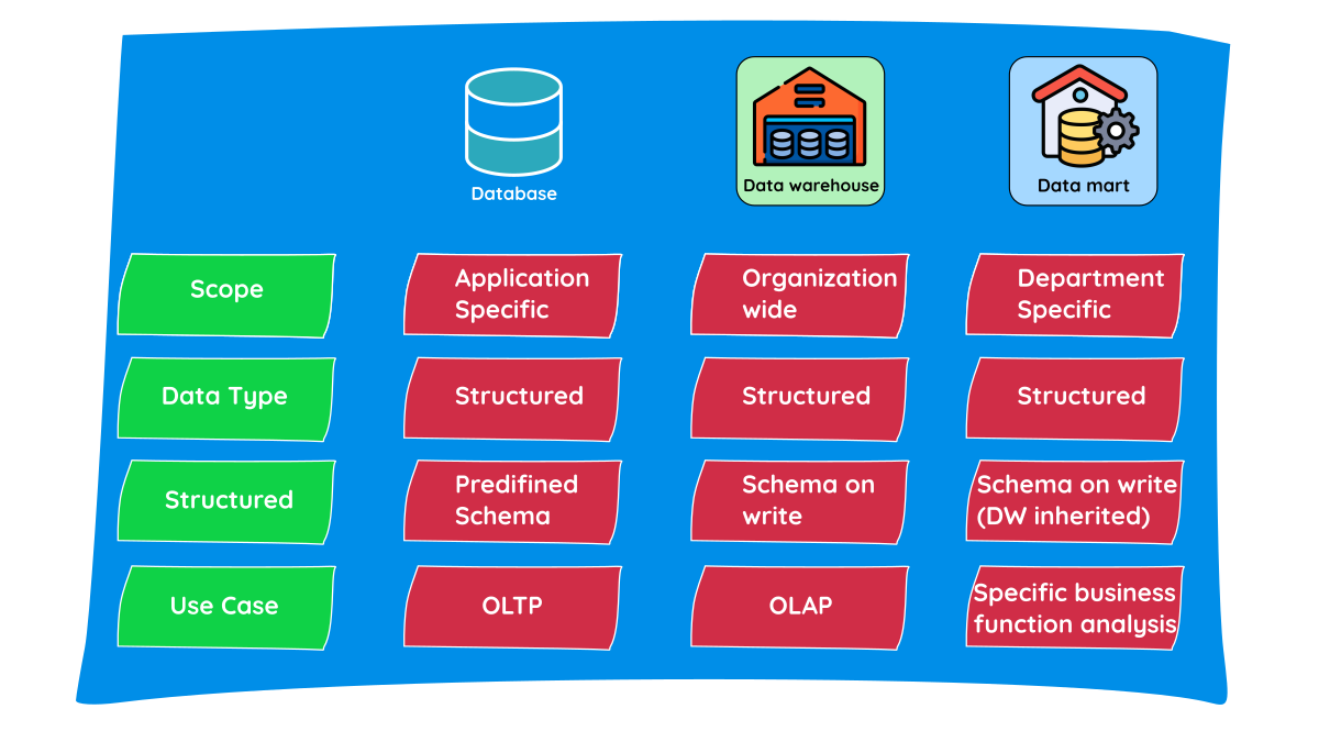
What is a Database?
A database is an organized collection of structured information, or data, typically stored electronically in a computer system. It is designed to store, manage, and retrieve data efficiently. It is usually designed to handle OLTP, i.e. for example, backend of application at counter of food store.
Note: We are not talking from hardware perspective, but how when these terms are used in data engineering domain.
What is a Data Warehouse?
A data warehouse is a centralized repository designed to store integrated data from multiple sources for analytical and reporting purposes. It supports historical analysis, business intelligence, and decision-making. Now, this can be a database, a lakehouse in databricks/spark etc. depending on requirements.
What is a Data Mart?
A data mart is a focused subset of data warehouse designed to meet the needs of a specific department or business function. It contains only the data relevant to that department.
Database vs Data Warehouse vs Data Mart
| Feature | Database | Data Warehouse | Data Mart |
|---|---|---|---|
| Purpose | Stores current operational data | Central repository for historical, analytical data | Focused subset of data warehouse |
| Model | ER model (normalized) | Dimensional/Star schema | Star schema |
| Users | Application users, developers | Analysts, BI professionals | Department users |
| Scope | Enterprise-wide transactions | Enterprise-wide analytics | Department-specific (e.g., Sales) |
| Update Frequency | Real-time or near real-time | Batch/ETL-driven | Batch |
Now lets look at the core concepts in datawarehousing and dimensional modelling.
What is a Data Warehouse
Imagine sufficiently large company wants any insights regarding how their comapny is performing (KPIs) or want to dig into some data because something's gone wrong or want to implement some ML usecase. They cannot go and query their EPR/CRMs/APIs or whatever their data source is everytime, this practice won't sustain.
That's why a data warehouse is necessary. As we discussed earlier, its a centralized repository designed to store integrated data from multiple sources for analytical and reporting purposes. It supports historical analysis, business intelligence, and decision-making.
Key Features
- Subject-oriented
- Integrated
- Time-variant
- Non-volatile
Data warehouses are optimized for reading large volumes of data unlike OLTP, becuase once the datawarehouse is in place, its written as per the refresh frequency, but is read quite frequently - by BI reports that get refreshed, ad-hoc queries by business users, downstream jobs. Targeted use cases are like trend analysis, forecasting, and executive dashboards etc.
In a very simple language, data warehouse built by kimball methodology is collection of fact and dimension tables modelled by business on top of which BI reports are built. Modelling in simple terms, is deciding what facts and dimensions should be created and what columns should those tables have.
Data Warehouse vs Lakehouse
Traditional data warehouses were prominently built using RDBMS systems like SQL Server, Oracle DB etc. Modern data wareshousing is done using 'lakehouses', you can find detailed information about it here.
| Feature | Data Warehouse | Lakehouse |
|---|---|---|
| Storage | Expensive DB (SQL Server, Teradata) | Cheap object storage (S3, ADLS) |
| Data type | Structured only | All types |
| Cost | High | Low |
| Tools | SSIS, Informatica | Spark, Databricks, ADF |
| Scalability | Limited (vertical scaling) | Massive (horizontal scaling) |
Data Modelling is done in similar way in both; the difference is in implementation
Two Approaches to Data Warehousing
There are two major approaches to data warehousing:
Inmon (Top-Down):
- Enterprise-wide data warehouse first
- Normalized data model (3NF)
- Data Marts created later
Kimball (Bottom-Up):
- Start with business-focused data marts
- Use dimensional modeling (star schemas)
- Integrate via conformed dimensions
Kimball’s method is popular - faster delivery, easier for business users, and good for iterative development
Kimball’s Dimensional Modeling
Dimensional modeling is a technique to structure data to be intuitive and performant for querying.
Two key components:
- Fact Tables (quantitative metrics)
- Dimension Tables (contextual attributes)
Goal: Create fact and dimension tables to make the data easy to understand and efficient to analyze.
High-Level Kimball Process
- Identify Business Process: Example: Orders, Payments, Shipments, Inventory -> This defines the scope of your fact table
Don't just build a generic
Fct_Salestable. Ask the stakeholders if they care about the checkout process, the shipping process, or returns. Each distinct business event gets its own fact table. Why? Because the process dictates the physical reality you are modeling. Once you isolate the specific process (e.g., "Customer pays for cart"), the raw columns naturally reveal themselves (transaction ID, payment method, tax amount). If you mix processes like adding shipping dates to a checkout fact - your data model will inevitably become a nightmare of NULL values and tangled logic. - Declare the Grain: What does one row in the fact table represent? Ex: one row per line item of transaction.
Business users always ask for aggregated data upfront ("I want to see monthly sales"). Push back. The grain is the single most critical decision in your entire warehouse design. If you get it wrong, your data is fundamentally broken for future use cases. If you declare the grain as "daily sales per store," but tomorrow marketing asks for "morning vs. evening sales," you are completely stuck. Always store data at the lowest possible atomic level (like one row per scanned barcode at the register) to future-proof your analytics. You can always aggregate up, but you can never drill down.
- Identify Dimensions: Who, what, where, when, how; ex: Customer, Product
Listen closely for the word "by" in meetings. "I want to see sales by store, by date, by customer". Those are your dims. A robust dimension table shouldn't just have an ID and a Name; it should be incredibly wide, packed with every descriptive attribute (category, sub-category, manager name, region) you can find. This empowers business users to slice and dice the metrics without writing complex SQL or submitting Jira tickets for new columns. Make sure these are conformed—meaning you use the exact same
DimCustomertable across all your fact tables to prevent data silos. - Identify Facts (Measures): Numeric, additive metrics
Keep these purely additive (like
Quantity,Sales_Amount). A fact must be true to the grain you just declared. If the grain is one line item on a receipt, the fact is the exact dollar amount for that specific item, not the total receipt amount. Furthermore, strictly separate additive facts from non-additive calculations (likeProfit_Margin). Calculate percentages on the fly in Power BI or your semantic layer. This guarantees that when a CEO looks at a high-level dashboard and an analyst looks at a granular report, the underlying numbers always match perfectly. - Design Star Schema (Logical Model): Central fact table + surrounding dimensions
Grab a whiteboard. Put the fact table in the middle and draw lines out to your dims. Do not skip this step and jump straight into coding. This diagram is your contract with the business. When stakeholders see how the central process connects to the entities they care about, they will immediately spot missing requirements. ("Wait, where is the promotion code?") Fixing it on the whiteboard takes five minutes; fixing it in production takes three weeks.*
- Define Keys & SCD Strategy: Surrogate keys, SCD
Never trust source system IDs (Natural Keys). Systems change and IDs get recycled, which will break your joins. Generate integer Surrogate Keys. Also, ask the hard questions: "If a user moves from Pune to Mumbai, do you want their past sales to show as Pune or Mumbai?" SCD Type 2 (history tracking) is what makes a warehouse vastly superior to a simple database replica, allowing true point-in-time reporting. But it is expensive to compute. Apply Type 2 only to critical attributes (like Region) and stick to Type 1 (overwrite) for trivial attributes (like a phone number).
- Source-to-Target Mapping: Column-level mapping, transformations, business rules
This is the unglamorous but necessary reality of data engineering. Source systems are usually a mess of obscure column names (like
usr_fld_12) and inconsistent data types. Your mapping document is the blueprint that translates that chaos into your pristine star schema. It is also where you define hard rules for data anomalies—what happens when a sale arrives without a valid customer ID? (Hint: you assign a default "-1" Unknown Customer SK). - Physical Model Design: Data types, Partitioning, Indexing (if warehouse), file formats
A logical star schema is useless if it's slow. The logical model tells you what the data means; the physical model dictates how fast you can read it. Are you on Synapse? Databricks? Fabric? If you partition a massive table by
Order_Datebut 90% of your queries filter byCustomer_ID, performance will tank. Figure out your partitioning strategy, file formats (Parquet/Delta), and things like Z-Ordering or Liquid Clustering to minimize data scanning. - ETL / ELT Design
Build the automated pipelines (ADF, Databricks, Airflow). Modern ELT emphasizes doing the heavy lifting within the warehouse (using tools like dbt) rather than on external servers. Focus heavily on modularity and idempotency here. If the API pulling exchange rates goes down, it shouldn't crash the pipeline loading customer addresses. Build resilient DAGs that gracefully handle failures, retry automatically, and ensure your dependencies are set so Dims always load before Facts.
- Build & Validate
What is Normalization and Denormalization?
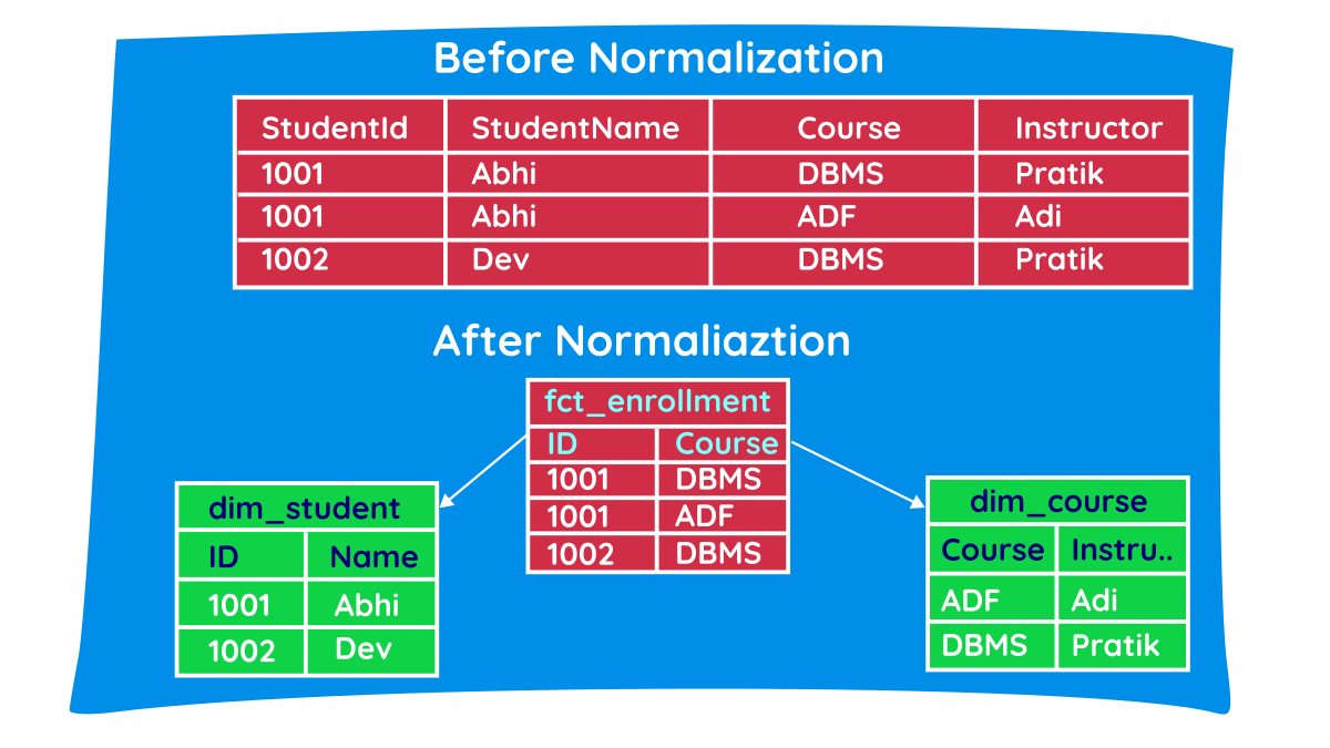
To understand why we design data warehouses the way we do, look at the visual above.
Before Normalization (Flat Table) Notice the redundancy: Student "Abhi" and Course "DBMS" are repeated. In an application database (OLTP), this is dangerous. If the instructor for DBMS changes, the application must update multiple rows. If one update fails, the database is corrupted with conflicting data.
After Normalization
We fix this by splitting the data into distinct entities (dim_student and dim_course) connected by a central mapping table. Now, if an instructor changes, we update exactly one row in the dim_course table. Zero risk of data corruption.
Software engineers achieve this normalized state by following three core rules:
- 1NF (First Normal Form): Atomic values only. One value per cell (no comma-separated arrays).
- 2NF (Second Normal Form): No partial dependencies. Every column must depend on the entire primary key, not just a piece of it.
- 3NF (Third Normal Form): No transitive dependencies. Every column must depend only on the primary key, not on other non-key columns (e.g., Zip Code dictates City and State, so they belong in a separate Location table).
The Data Engineering Reality (Denormalization) Strict 3NF is the gold standard for writing data safely in OLTP systems. However, Data Warehouses (OLAP) are built for reading data. Joining multiple normalized tables across a billion rows requires heavy network shuffling, which is incredibly slow.
Therefore, Data Engineers intentionally denormalize the data. We trade storage space, reintroducing controlled redundancy to build Star Schemas or One Big Tables (OBT) that allow massive analytical queries to return in milliseconds.
Normalization is critical in transactional systems to avoid data redundancy & prevent update/insert/delete anomaly
Normalization
- Method used in a database to reduce the data redundancy and data inconsistency
- Organizing data to reduce redundancy and improve data integrity.
- Achieved through splitting tables (1NF, 2NF, 3NF, etc.).
- Used in OLTP systems.
- Optimized for write/update/delete operations.
Denormalization
- Method used in a database to add the redundancy to execute the query quickly
- Combining data to reduce the number of joins.
- Intentional redundancy for performance.
- Used in OLAP/Data Warehousing.
- Optimized for read/query operations.
Why Denormalize in Data Warehousing?
- Queries are more predictable and faster.
- Simplifies reporting and analytics for business users.
Fact Tables
Store measurable, quantitative data Typically contain:
- Foreign keys to dimensions
- Metrics (e.g., sales amount, quantity)
Types of Fact Tables:
- Transactional
- Snapshot
- Accumulating
You can read more about the different types here
Granularity
- Level of detail represented by the fact table
- Example: Daily sales per store = fine grain, Monthly sales per region = coarse grain
- Why it matters: Impacts data volume, query speed, and usability.
Dimension Tables
Contain descriptive attributes that provide context to facts Example: Customer, Product, Time, Georgraphy
Characteristics:
- Textual and categorical
- Denormalized (in star schema)
Star Schema
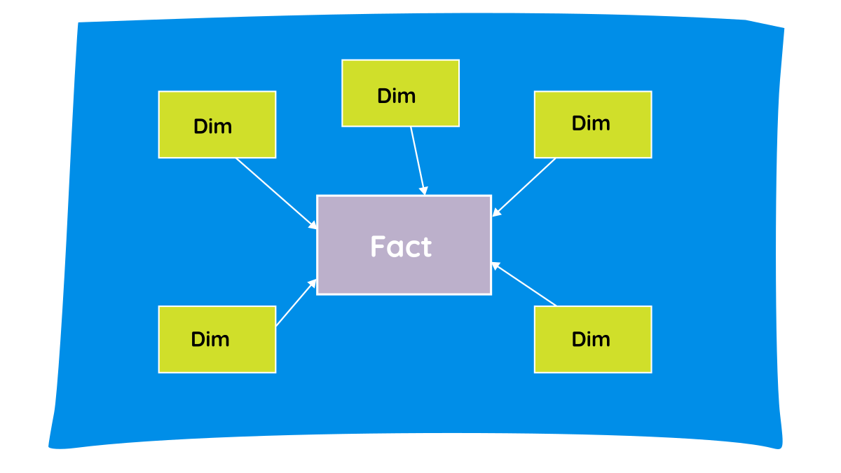
A simple, de-normalized structure
- Centered around a fact table
- Connected to multiple dimension tables
Pros:
- Fast query performance due to fewer & simple joins [dims are small, can be broadcasted + facts are narrow]
- Easy for business users
Notice the direction of arrows, they flow from dimension to fact. This signifies that data from dimension table will filter the data in fact table in BI reports (ex: PowerBI), never the other way around. This also tells us dimension tables primarily serve the purpose of slicing and dicing data in fact tables in reporting.
Snowflake Schema
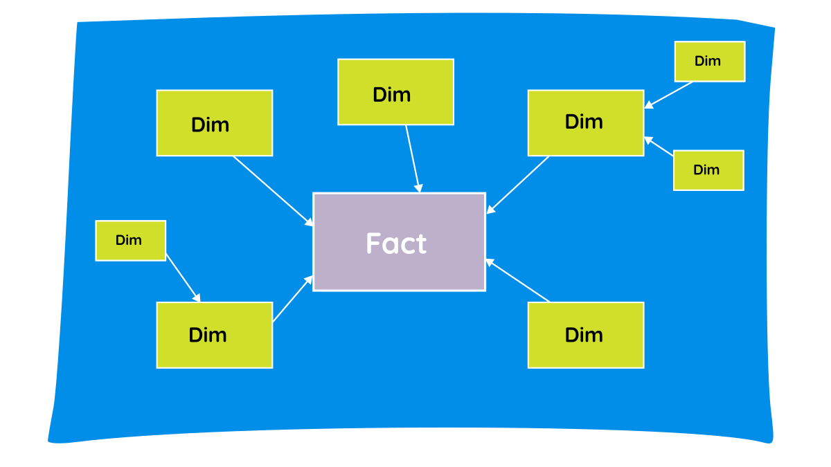
A normalized variant of the star schema
- Dimension tables are further split into sub-dimensions
- Star schema stores all hierarchy data in one wide table (DimProduct), a Snowflake schema normalizes it by splitting those hierarchies into separate, linked tables (Product → SubCategory → Category).
Pros:
- Reduces data redundancy
- Better data integrity
Cons:
- More complex for querying
It saves a tiny bit of storage space, but it forces your database to perform three separate JOINs just to find out the Category of a sold item. That extra "hop" is exactly why it looks like a snowflake on a diagram, and exactly why it runs slower in an analytical data warehouse.
Slowly Changing Dimensions (SCD)
- Type 0 – Fixed: Don’t change
- Type 1 – Overwrite: Replace old data
- Type 2 – History: Add a new row
- Type 3 – Previous Value: Add new column for change
Note: Type 2 is most common—when customer address changes, we add a new row to track history.
When to use SCD 1 & SCD 2?
SCD1 if business only cares about latest value
SCD2 if historical tracking is needed.
Real Scenario: If a customer moves from Pune to Mumbai, should old sales show Pune or Mumbai? Regulatory / Financial Impact? -> If YES → almost always Type 2
Types of Keys in Dimensional Modeling
| Key Type | Purpose | Example |
|---|---|---|
| Primary Key | Uniquely identifies a record in a table | Customer_ID in Customer table |
| Foreign Key | References primary key in another table | Customer_ID in Sales fact table |
| Surrogate Key | Artificial unique identifier (e.g., integer) | Product_SK (auto-incremented) |
| Natural Key | Real-world identifier from source systems | SSN, Email |
| Unique Key | Enforces uniqueness on a column or set of columns | Email in Customer table |
| Alternate Key | Any candidate key not selected as primary key | National_ID if Customer_ID is primary |
Note: Surrogate keys are preferred in dimensional modeling: avoid source system dependencies and simplify SCD handling. Natural keys can change (e.g., phone number), which makes them unstable.
Surrogate keys
- What is a Surrogate Key? A surrogate key (SK) is an artificial, system-generated unique identifier (usually an integer) used to uniquely identify a record in a dimension table.
- Why NOT use Natural Keys directly? A natural key can change due to business or system reasons -> if PK is used, it will be needed to be updated everywhere, but if SK is used, PK to be updated only in dim table
- Required for SCD type 2 as updated records will have same PK
- Performance Optimization: Surrogate keys are typically Ints ((4 or 8 bytes)
Best Practices in Dimensional Modeling
- Start with business process, not data
- Define clear grain early
- Avoid junk dimensions (unless needed)
- Use surrogate keys
- Handle SCDs thoughtfully
- Validate with real queries
Resources & Further Reading
- The Data Warehouse Toolkit – Ralph Kimball
- Kimball Group’s website
- Blogs: Brent Ozar, Fivetran, Databricks
Interview Questions on Data Warehousing
If you are preparing for a Data Engineering interview, expect to be tested heavily on these concepts. Here are a few advanced questions to practice:
1. When would you choose to build a Snowflake schema instead of a Star schema?
- Answer: I always default to a Star schema because read performance is the priority in a data warehouse, and fewer joins mean faster queries. However, I would choose a Snowflake schema if a specific dimension has massive, unwieldy data redundancy that is causing severe storage issues or making updates difficult. For example, if a
DimProducttable has millions of rows and we need to frequently update category-level attributes, separatingDimCategoryinto its own table (snowflaking) makes sense to enforce strict data integrity and simplify updates. The trade-off, of course, is that we pay for it with more complex, slower joins at query time.
2. Explain the exact difference between SCD Type 1 and Type 2. When would a business mandate Type 2?
- Answer: The core difference is historical tracking. SCD Type 1 simply overwrites the existing record; if a customer moves from New York to California, their state is updated to California, and the historical context is permanently lost. SCD Type 2 inserts a completely new row for that customer with the new state, while marking the old row as inactive using
Effective_Start_Date,Effective_End_Date, and anIs_Currentflag. A business will mandate Type 2 whenever accurate point-in-time analytics, financial reporting, or regulatory compliance is required. For instance, if we are auditing regional sales from 2023, the business needs to know where the customer lived at the time of the sale, not where they live today.
3. Why is it dangerous to use Natural Keys directly in your Fact Tables?
- Answer: It is dangerous because natural keys, like an email address, SSN, or a source system ID are fundamentally unstable. They can change, be reassigned, or get recycled by the source system. If a natural key changes and you have used it in your Fact table, you are forced to run a massive, highly expensive
UPDATEstatement across potentially billions of rows just to maintain referential integrity. By generating an artificial, integer-based Surrogate Key, you isolate that instability. If a user's email changes, you only update that single row in the Dimension table. The Surrogate Key remains the same, leaving the massive Fact table completely untouched and performant.
TL;DR / Summary
At its core, a Data Warehouse exists to turn chaotic operational data into structured analytical insights.
While OLTP systems use highly normalized models to handle fast day-to-day transactions safely, Data Warehouses use Dimensional Modeling (usually the Kimball Star Schema) to optimize for massive, read-heavy analytical queries. By establishing a clear grain, decoupling facts from dimensions, utilizing Surrogate Keys, and properly tracking historical changes via SCDs, we build data structures that are incredibly intuitive for analysts and highly performant for BI tools.
- Kimball’s approach is practical and business-focused
- Dimensional modeling makes data easy to understand and analyze
- Star schema = simplicity & speed
- Use conformed dimensions to scale